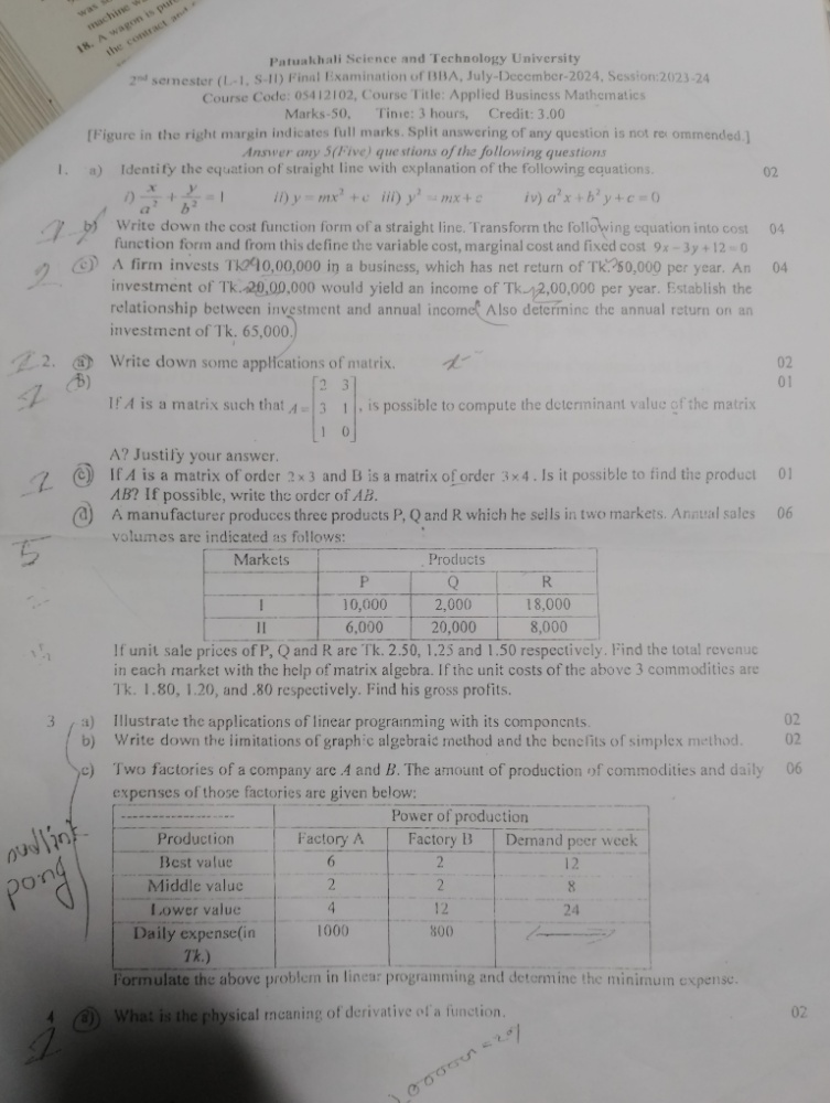
Set 1

Question 1

a) Identification of Straight Line Equations

• i) $\frac{x^2}{a^2}+\frac{y^2}{b^2}=1$: Not a straight line. This is the standard equation of an ellipse centered at the origin, as both variables are squared (degree 2).
• ii) $y=m{x}^2+c$: Not a straight line. This represents a parabola opening vertically, as $x$ has a degree of 2.
• iii) $y^2=mx+c$: Not a straight line. This represents a parabola opening horizontally, as $y$ has a degree of 2.
• iv) $a^{2}x+b^{2}y+c=0$: This is the equation of a straight line. It is a general linear equation in two variables where both $x$ and $y$ are of first degree (degree 1).

b) Cost Function Form and Transformation

The cost function form of a straight line is written as:

Where:

• $x$ = output quantity (number of units)
• $y$ or $C(x)$ = total cost
• $v$ or $m$ = variable cost per unit (marginal cost)
• $F$ or $c$ = fixed cost

Given linear equation:

Transforming into cost function form by solving for $y$:

From this cost function $C(x)=3x+4$:

• Variable Cost ($VC$): $3x$ (the component dependent on output quantity $x$)
• Marginal Cost ($MC$): $\frac{dC}{dx}=3$ (the slope, representing the cost added by producing one additional unit)
• Fixed Cost ($FC$): $4$ (the constant term, representing cost incurred when $x=0$)

c) Investment vs. Income Linear Model

Let:

• $x$ = investment amount (in Tk.)
• $y$ = annual income / return (in Tk.)

We are given two coordinate points $(x_1,y_1)$ and $(x_2,y_2)$:

• Point 1: $(10,00,000,50,000)$
• Point 2: $(20,00,000,2,00,000)$

Step 1: Find the slope (m)

Step 2: Establish the linear equation

Using the point-slope formula $y-y_1=m(x-x_1)$:

Relationship between investment and annual income:

Step 3: Determine return on investment of Tk. 65,000

Substitute $x=65,000$:

The annual return on an investment of Tk. 65,000 is -Tk. 90,250 (representing a net loss of Tk. 90,250 due to fixed operating costs/overhead).

Question 2

a) Applications of Matrices in Business and Economics

1. Revenue and Cost Calculation: Multi-product pricing and sales volume analysis across multiple retail markets.
2. Input-Output Analysis: Modeling inter-industry dependencies and production requirements in macroeconomics (Leontief models).
3. Linear Programming: Solving complex resource allocation problems via the Simplex method.
4. Markov Chains: Forecasting consumer market share transitions and credit risk defaults over time.

b) Determinant Evaluation of Matrix A

Matrix $A=\left[\begin{array}{cc}2& 3\\ 3& 1\\ 1& 0\end{array}\right]$ is of dimension $3\times 2$ (3 rows, 2 columns).

Answer: No, it is not possible to compute the determinant of $A$.

Justification: Determinants are mathematically defined only for square matrices (where the number of rows equals the number of columns, $n\times n$). Since $A$ is a rectangular matrix ($3\times 2$), its determinant does not exist.

c) Matrix Product AB and Dimension

• Order of matrix $A$: $2\times 3$
• Order of matrix $B$: $3\times 4$

Is product $AB$ possible? Yes. The number of columns in $A$ (3) equals the number of rows in $B$ (3).

Order of $AB$: $2\times 4$

d) Market Revenue and Gross Profit via Matrix Algebra

Given sales matrix $S$ ($2\times 3$):

Selling price column vector $P$ ($3\times 1$):

Unit cost column vector $C$ ($3\times 1$):

1. Total Revenue in Each Market

Revenue matrix $R=S\times P$:

• Market I Revenue:$$$$$$$$$$$$$$$$

R = \begin{bmatrix} 54,500 \ 52,000 \end

U = \begin{bmatrix} 2.50 - 1.80 \ 1.25 - 1.20 \ 1.50 - 0.80 \end{bmatrix} = \begin{bmatrix} 0.70 \ 0.05 \ 0.70 \end

\Pi = \begin{bmatrix} 10,000 & 2,000 & 18,000 \ 6,000 & 20,000 & 8,000 \end{bmatrix} \begin{bmatrix} 0.70 \ 0.05 \ 0.70 \end

\Pi_1 = (10,000 \times 0.70) + (2,000 \times 0.05) + (18,000 \times 0.70) = 7,000 + 100 + 12,600 = 19,700\text{ Tk.}
$$

• Market II Gross Profit:$$$$$$$$$$$$$$$$

a) Applications and Components of Linear Programming

Key Applications

1. Production Mix: Finding the profit-maximizing output combination subject to machine and labor constraints.
2. Cost Minimization / Transportation: Minimizing distribution expenses across supply chain networks.

Key Components

1. Decision Variables: Unknown quantities to be determined ($x_1,x_2,\dots$).
2. Objective Function: The mathematical expression to be maximized (e.g., Profit) or minimized (e.g., Cost).
3. Constraints: Structural inequalities representing resource limits, capacity, or demand requirements.
4. Non-negativity Conditions: Constraints ensuring real-world variables remain non-negative ($x_i\ge 0$).

b) Graphical Method Limitations vs. Simplex Method Benefits

Limitations of Graphical Method

1. Limited to problems with at most two decision variables ($x_1,x_2$).
2. Inaccurate for determining non-integer or fractional coordinate intersections manually.

Benefits of Simplex Method

1. Solves linear programming problems involving any number of decision variables and constraints.
2. Provides dual values (shadow prices) for optimal resource valuation and sensitivity analysis.

c) LPP Formulation and Optimization

Let:

• $x_1$ = number of days Factory A operates per week
• $x_2$ = number of days Factory B operates per week

Objective Function

Minimize total daily operational expense $Z$:

Demand Constraints

1. Best value commodity: $6x_1+2x_2\ge 12⟹3x_1+x_2\ge 6$
2. Middle value commodity: $2x_1+2x_2\ge 8⟹x_1+x_2\ge 4$
3. Lower value commodity: $4x_1+12x_2\ge 24⟹x_1+3x_2\ge 6$
4. Non-negativity: $x_1\ge 0,x_2\ge 0$

Corner Point Evaluation of Feasible Region

Boundary line intersections:

1. $3x_1+x_2=6$
2. $x_1+x_2=4$
3. $x_1+3x_2=6$

Intersection points defining the boundary of the feasible region:

• Point A: Intersection of $x_1=0$ and $3x_1+x_2=6⟹(0,6)$
• Point B: Intersection of $3x_1+x_2=6$ and $x_1+x_2=4$: Subtracting gives $2x_1=2⟹x_1=1,x_2=3⟹(1,3)$
• Point C: Intersection of $x_1+x_2=4$ and $x_1+3x_2=6$: Subtracting gives $2x_2=2⟹x_2=1,x_1=3⟹(3,1)$
• Point D: Intersection of $x_2=0$ and $x_1+3x_2=6⟹(6,0)$

Objective Function Values at Corner Points

Conclusion: Minimum expense is Tk. 3,400, achieved when Factory A operates for 1 day and Factory B operates for 3 days per week.

Question 4

a) Physical Meaning of Derivative

The derivative of a function $y=f(x)$, denoted as $\frac{dy}{dx}$ or $f^{\prime }(x)$, represents the instantaneous rate of change of $y$ with respect to $x$.

• Geometrically: It is the slope of the tangent line to the curve at a given point.
• Economically: It measures marginal values, such as marginal cost ($\frac{dC}{dq}$) or marginal revenue ($\frac{dR}{dq}$), indicating the rate at which total output changes when input changes by one unit.

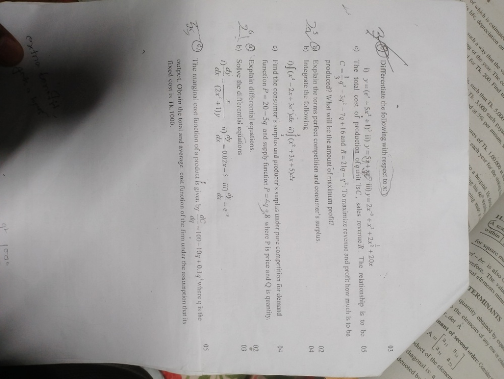
b) Differentiation Problems

i) $y=(e^x+5x^2+1{)}^3$

Using Chain Rule $\frac{d}{dx}[u^n]=n{u}^{n-1}\cdot u^{\prime }$:

ii) $y=\frac{5x^2+2}{x^3+1}$

Using Quotient Rule $\frac{d}{dx}\left[\frac{u}{v}\right]=\frac{u^{\prime }v-u{v}^{\prime }}{v^2}$:

iii) $y=2x^3+x^2+2x^2+20x$

Simplify terms ($x^2+2x^2=3x^2$):

c) Revenue and Profit Maximization

Given:

1. Revenue Maximization

First-order condition ($\frac{dR}{dq}=0$):

Second-order condition:

Maximum Revenue:

2. Profit Maximization

First-order condition ($\frac{d\mathrm{\Pi }}{dq}=0$):

Using the quadratic formula $q=\frac{-b\pm \sqrt{b^2-4ac}}{2a}$:

Second-order condition:

At $q=7.66$:

Maximum Profit:

Question 5

a) Concepts Explanation

• Perfect Competition: A market structure featuring numerous small buyers and sellers, standardized products, perfect mobility of resources, zero market entry/exit barriers, and perfect information. Individual firms are price takers ($P=MR=AR$).
• Consumer's Surplus: The economic benefit measured by the total area between the demand curve and the market price line up to the quantity purchased. It represents the difference between total willingness to pay and total actual expenditure:$$$$$$$$

i) $\int (x^4-2x+3e^x)dx$

ii) ${\int }_1^2(x^2+3x+5)dx$

At upper limit $x=2$:

At lower limit $x=1$:

Difference:

c) Consumer's Surplus and Producer's Surplus

Given:

• Demand: $P_d=20-5q$
• Supply: $P_s=4q+8$

1. Equilibrium Point $(q_0,P_0)$

2. Consumer's Surplus (CS)

3. Producer's Surplus (PS)

Question 6

a) Differential Equations Concept

A differential equation is a mathematical equation relating an unknown function to one or more of its derivatives. In economics and business, differential equations model continuous growth dynamics, price adjustment models over time, continuous compounding, and total cost recovery from marginal functions.

b) Solving Differential Equations

i) $\frac{dy}{dx}=\frac{x}{(2x^2+1)y}$

Separating variables:

Integrating both sides:

ii) $\frac{dy}{dx}=0.02x-5$

Integrating both sides:

iii) $\frac{dy}{dx}=e^x$

Integrating both sides:

c) Total Cost and Average Cost Functions

Given marginal cost function:

Fixed cost $FC=1000$ (when $q=0$, $C(0)=1000$).

1. Total Cost Function $C(q)$

Since $C(0)=1000⟹K=1000$.

Total Cost Function:

2. Average Cost Function $AC(q)$

Set 2

Question 1

a) Standard Form of the Cost Equation

The standard form of a linear cost equation is written as:

Where:

• $x$ = Quantity of output produced (units)
• $y$ or $C(x)$ = Total cost
• $v$ or $m$ = Variable cost per unit (marginal cost)
• $F$ or $c$ = Total fixed cost

b) Conditions for Parallel and Perpendicular Straight Lines

Let two straight lines have marginal costs (slopes) $m_1$ and $m_2$:

• Parallel Lines Condition: The two lines are parallel if their slopes are equal:$$$$$$$$$$$$$$$$

Given straight line equation:

Transform into standard cost function form $y=mx+c$ by solving for $y$:

From this cost equation $C(x)=\frac{2}{3}x+\frac{5}{3}$:

1. Marginal Cost ($MC$): Slope of the equation $m=\frac{\mathbf{2}}{\mathbf{3}}$
2. Fixed Cost ($FC$): $y$-intercept $c=\frac{\mathbf{5}}{\mathbf{3}}$
3. Total Cost ($TC$) Function: $\mathbf{y}\mathbf{=}\frac{\mathbf{2}}{\mathbf{3}}\mathbf{x}\mathbf{+}\frac{\mathbf{5}}{\mathbf{3}}$

Variable Cost when $x=100$ units

Variable cost function $VC(x)=v\cdot x=\frac{2}{3}x$

d) Order Processing Cost Linear Model

Let:

• $x$ = Number of orders processed
• $y$ = Processing money / total cost (in Tk.)

Given data points $(x_1,y_1)$ and $(x_2,y_2)$:

• Point 1: $(100,4000)$
• Point 2: $(200,6000)$

Step 1: Find the slope / marginal cost (m)

• Marginal Cost: Tk. 20 per order

Step 2: Derive the relation between processing money and number of orders

Using point-slope formula $y-y_1=m(x-x_1)$:

• Linear Relation: $\mathbf{y}\mathbf{=}\mathbf{20}\mathbf{x}\mathbf{+}\mathbf{2000}$

Step 3: Total cost for 400 orders

Substitute $x=400$:

Question 2

a) Properties and Applications of Determinants

Three Properties of Determinants

1. Determinant of Transpose: Transposing a matrix does not change its determinant: $|A^T|=|A|$.
2. Row/Column Interchange: Interchanging any two rows or columns changes the sign of the determinant.
3. Scalar Multiplication: Multiplying a single row or column of a matrix by a scalar $k$ multiplies the value of the determinant by $k$.

Applications

• Solving systems of linear equations using Cramer's Rule.
• Calculating matrix inverses ($A^{-1}=\frac{1}{|A|}\text{adj}(A)$).
• Testing singularity ($|A|=0$) to verify if a system has a unique solution.

b) System of Linear Equations via Cramer's Rule

Given system:

Writing system as matrix $AX=B$:

Step 1: Calculate Determinant $|D|$

Expand $|A|$ along Row 3:

Step 2: Calculate $|D_x|$

Replace Column 1 with $B$:

Expand along Row 3:

Step 3: Calculate $|D_y|$

Replace Column 2 with $B$:

Expand along Row 1:

Step 4: Calculate $|D_z|$

Replace Column 3 with $B$:

Expand along Row 3:

Step 5: Solve for variables

c) Examples of Matrices

• Row Matrix: A matrix with only 1 row:$$$$$$$$$$$$$$$$$$$$$$$$

Let prices of share types $x,y,z$ be represented by vector $P=\left[\begin{array}{c}x\\ y\\ z\end{array}\right]$.

From investor purchases:

• Investor A: $2x+5y+3z=480$
• Investor B: $4x+3y+6z=760$
• Investor C: $1x+4y+10z=710$

Matrix system $AX=B$:

Step 1: Find Inverse $A^{-1}$

Cofactors of $A$:

Step 2: Compute $X=A^{-1}B$

• For $x$:$$$$$$$$$$$$$$$$$$$$$$$$

a) Applications of Linear Programming

Linear programming optimizes real-world operational problems such as product mix optimization, supply chain transportation cost minimization, portfolio asset allocation, and labor scheduling constraints.

b) Graphical Method Limitations vs. Simplex Method Benefits

• Graphical Method Limitations: Limited strictly to 2 decision variables ($x,y$) and relies on visual estimation of intersections.
• Simplex Method Benefits: Solves linear optimization problems across arbitrary numbers of decision variables and constraints while generating dual values (shadow prices).

c) Optimization via Simplex Method

Maximize: $Z=4x+6y$

Subject to constraints:

1. $x+2y\le 8$
2. $2x+y\le 8$
3. $4x-2y\le 2$
4. $x,y\ge 0$

Convert to Standard Form with Slack Variables $(s_1,s_2,s_3)$

Initial Simplex Tableau

Most negative indicator in $Z$-row is $-6$ (column $y$). Leaving variable is $s_1$ (minimum ratio $4$). Pivot element = 2 (Row 1, Column 2).

Iteration 1

Divide Row 1 by 2:

Perform row operations:

• $R_2^{\prime }=R_2-1(R_1^{\prime })=[\frac{3}{2},0,-\frac{1}{2},1,0,4]$
• $R_3^{\prime }=R_3+2(R_1^{\prime })=[5,0,1,0,1,10]$
• $Z^{\prime }=Z+6(R_1^{\prime })=[-1,0,3,0,0,24]$

Most negative indicator in $Z$-row is $-1$ (column $x$). Leaving variable is $s_3$ (minimum ratio $2$). Pivot element = 5 (Row 3, Column 1).

Iteration 2

Divide Row 3 by 5:

Perform row operations:

• $R_1^{″}=R_1^{\prime }-\frac{1}{2}(R_3^{″})=[0,1,\frac{2}{5},0,-\frac{1}{10},3]$
• $R_2^{″}=R_2^{\prime }-\frac{3}{2}(R_3^{″})=[0,0,-\frac{4}{5},1,-\frac{3}{10},1]$
• $Z^{″}=Z^{\prime }+1(R_3^{″})=[0,0,\frac{16}{5},0,\frac{1}{5},26]$

Final Optimal Tableau

Since all $Z$-row indicators are $\ge 0$, optimal solution is reached.

• Optimal Variables: $x=\mathbf{2},y=\mathbf{3}$
• Maximum Objective Value: $Z_{\text{max}}=4(2)+6(3)=\mathbf{26}$

Question 4

a) Physical Meaning of Derivative

The derivative of a function $y=f(x)$ measures the instantaneous rate at which $y$ changes relative to $x$. Geometrically, it defines the slope of the tangent line at a point on the curve. In business applications, it yields marginal concepts such as marginal revenue, marginal cost, and elasticities.

b) Differentiation Problems

i) $y=e^x+2x+1$

ii) $y=5+x{e}^x$

Using the product rule on $x{e}^x$:

iii) $y=10x^{-1}+x^3+2x^2+20$

c) Profit Maximization and Specific Output Evaluation

Given:

• Cost: $C(x)=100+0.015x^2$
• Revenue: $R(x)=3x$

Profit function $\mathrm{\Pi }(x)=R(x)-C(x)$:

1. Maximizing Quantity $(x)$

First-order condition ($\frac{d\mathrm{\Pi }}{dx}=0$):

Second-order condition check:

2. Maximum Profit Amount

3. Profit when Output $x=120$

Question 5

a) Market Structure Comparison

• Perfect Competition: Market structure with infinite buyers and sellers trading identical, homogeneous products. Individual firms have no pricing power ($P=MR=AR$) and face zero barriers to entry/exit.
• Monopoly: Market structure with a single firm controlling the total supply of a unique product without close substitutes. The monopolist is a price setter facing a downward-sloping demand curve.

b) Total and Average Cost from Marginal Cost

Given marginal cost:

Fixed cost $FC=1000$ (i.e., $C(0)=1000$).

Total Cost Function $C(q)$

Since $C(0)=1000⟹K=1000$.

Average Cost Function $AC(q)$

c) Consumer's and Producer's Surplus

Given functions:

• Demand: $P=\frac{8}{Q+1}-2$
• Supply: $P=\frac{Q+3}{2}$

Step 1: Equilibrium Point $(Q_0,P_0)$

Since quantity $Q\ge 0$:

Step 2: Consumer's Surplus (CS)

Step 3: Producer's Surplus (PS)

Question 6

a) Definition of Differential Equations

A differential equation is an equation involving an unknown function and its derivatives with respect to one or more independent variables.

b) Solving Differential Equations

i) $\frac{dy}{dx}=\frac{1}{(2x+1)y}$

Separating variables:

Integrating both sides:

ii) $\frac{dy}{dx}=0.02y-5$

Separating variables:

Integrating both sides:

iii) $\frac{dy}{dx}=e^{-y}{e}^x$

Separating variables:

Integrating both sides:

c) Continuous Compounding Doubling Time

Given:

• Principal $P=10,000$
• Target Amount $A=20,000$ (doubling)
• Annual rate $r=4\mathrm{\%}=0.04$

Continuous compounding formula:

Taking natural logarithm ($\ln$) on both sides:

It will take approximately 17.33 years (or 17 years and 4 months) for the investment to double.

Set 3

Question 1

a) Coordinates of Points Dividing the Line Segment

Given two points $A(4,7)$ and $B(2,4)$, with ratio $m:n=3:5$.

1. Internal Division

Using the section formula for internal division $P(x,y)=(\frac{m{x}_2+n{x}_1}{m+n},\frac{m{y}_2+n{y}_1}{m+n})$:

• Internal Division Point: $(\frac{\mathbf{13}}{\mathbf{4}}\mathbf{,}\frac{\mathbf{47}}{\mathbf{8}})$ or $(3.25,5.875)$

2. External Division

Using the section formula for external division $Q(x,y)=(\frac{m{x}_2-n{x}_1}{m-n},\frac{m{y}_2-n{y}_1}{m-n})$:

• External Division Point: $(\mathbf{7}\mathbf{,}\frac{\mathbf{23}}{\mathbf{2}})$ or $(7,11.5)$

b) Unit Vector Parallel to Resultant Vector $\overrightarrow{R}$

Given vectors:

• ${\overrightarrow{r}}_1=2\hat{i}+4\hat{j}$
• ${\overrightarrow{r}}_2=-\hat{i}-2\hat{j}+3\hat{k}$

Step 1: Find Resultant Vector $\overrightarrow{R}={\overrightarrow{r}}_1+{\overrightarrow{r}}_2$